Convergence and Diagnostics • exnexSurv

Overview

This vignette shows a simple workflow for checking whether the sampler appears stable in practice. The package now supports multiple chains, including R-level parallel execution, so the examples below combine:

traceplots,
running means,
effective sample size approximations,
repeated fits with different seeds.

Simulate data

library(exnexSurv)
library(survival)
library(ggplot2)
library(bayesplot)

simulate_surv_data <- function(
  theta,
  sigma2,
  beta = NULL,
  n_per_group = 60,
  censor_min = 4,
  censor_max = 12,
  seed = NULL
) {
  if (!is.null(seed)) {
    set.seed(seed)
  }

  groups <- rep(seq_along(theta), each = n_per_group)
  age_std <- rnorm(length(groups), mean = 0, sd = 1)
  mean_log_time <- rep(theta, each = n_per_group)

  if (!is.null(beta)) {
    mean_log_time <- mean_log_time + beta * age_std
  }

  log_time <- rnorm(length(groups), mean = mean_log_time, sd = sqrt(sigma2))
  true_time <- exp(log_time)
  censor_time <- runif(length(groups), min = censor_min, max = censor_max)

  data.frame(
    time = pmin(true_time, censor_time),
    event = as.integer(true_time <= censor_time),
    group = factor(groups),
    age_std = age_std
  )
}

sim_data <- simulate_surv_data(
  theta = c(1.2, 1.7, 2.1),
  sigma2 = 0.20,
  beta = -0.35,
  n_per_group = 60,
  seed = 6841
)

mean(sim_data$event)
#> [1] 0.6777778

Fit multiple chains

fit <- exnex_surv(
  Surv(time, event) ~ group + age_std,
  data = sim_data,
  iter = 3000,
  warmup = 1000,
  chains = 2,
  parallel_chains = 2,
  seed = 6841
)

print(fit, show_trace = FALSE)
#> <exnex_surv model>
#> Draws: 4000 total post-warmup samples
#>        2000 post-warmup samples per chain
#> Groups: 3 | Covariates: 1 
#> MCMC: iter = 3000 , warmup = 1000 , chains = 2 
#> 
#>  parameter       mean         sd        q05        q50        q95
#>    theta_1  1.2463566 0.06462694  1.1403574  1.2466079  1.3532442
#>    theta_2  1.7120960 0.06780666  1.6006020  1.7114203  1.8234427
#>    theta_3  2.1643972 0.07989574  2.0348217  2.1631064  2.2992832
#>     beta_1 -0.3834375 0.04700082 -0.4604095 -0.3846512 -0.3059669
#>     sigma2  0.2321148 0.03015053  0.1875849  0.2298443  0.2862142

This fit stores all post-warmup draws in one table. With chains = 2, each chain contributes the same number of post-warmup iterations, so chain-aware diagnostics can reconstruct the original chain layout from the total row count.

Traceplots

plot(fit, ask = FALSE)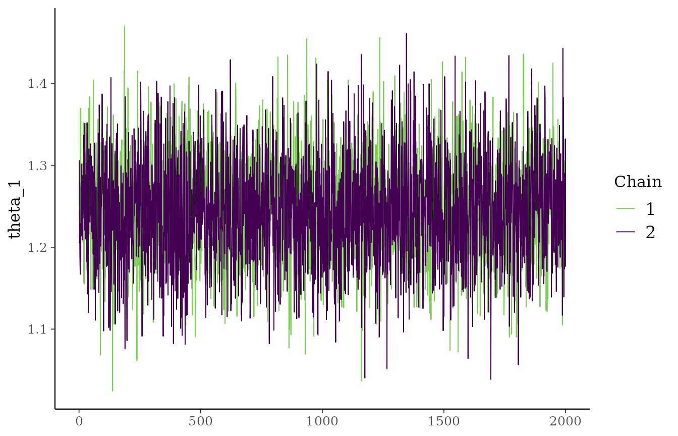

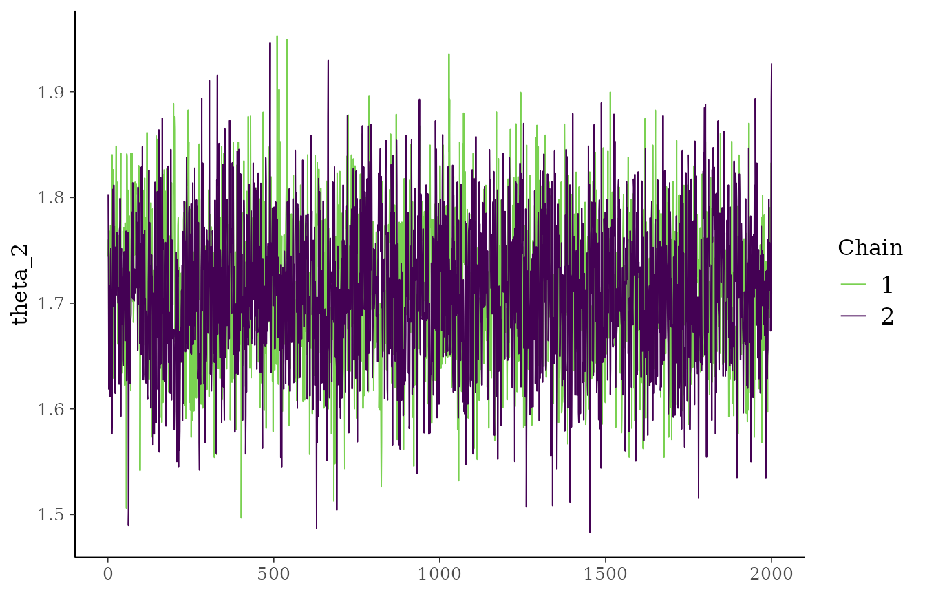
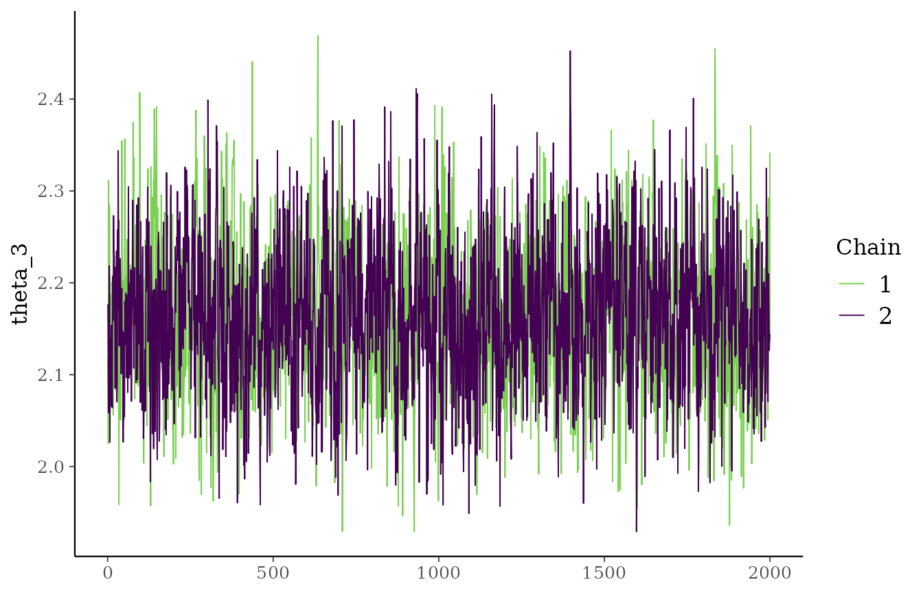
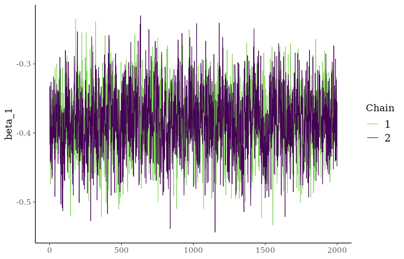
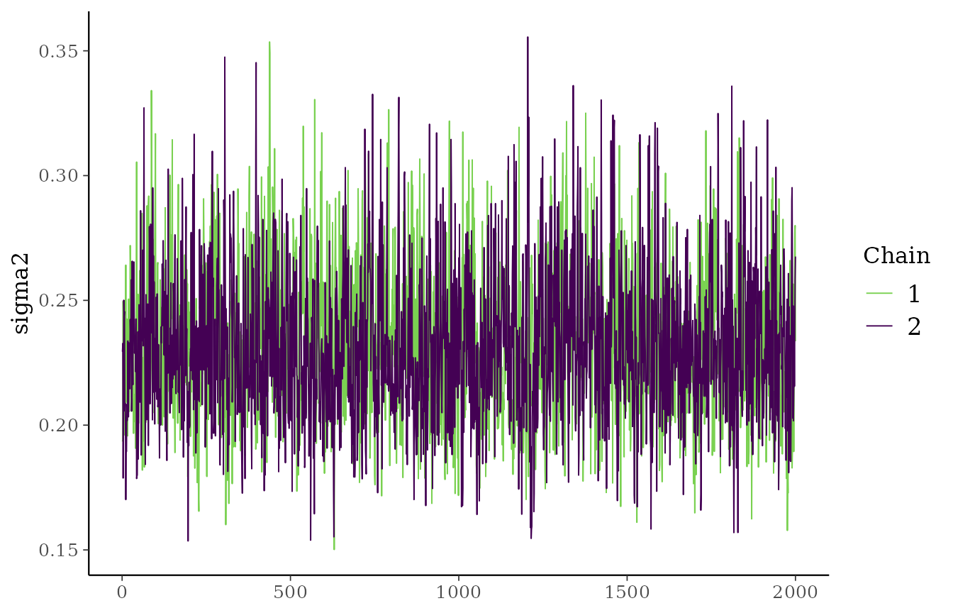
A healthy traceplot usually shows noisy fluctuations around a roughly stable level rather than long drifts or very sticky behavior.

Running means

running_mean_df <- do.call(
  rbind,
  lapply(colnames(fit$draws), function(param) {
    values <- fit$draws[[param]]
    data.frame(
      iteration = seq_along(values),
      running_mean = cumsum(values) / seq_along(values),
      parameter = param
    )
  })
)

ggplot(running_mean_df, aes(iteration, running_mean)) +
  geom_line() +
  facet_wrap(~ parameter, scales = "free_y") +
  labs(
    title = "Running posterior means",
    x = "Post-warmup iteration",
    y = "Running mean"
  )

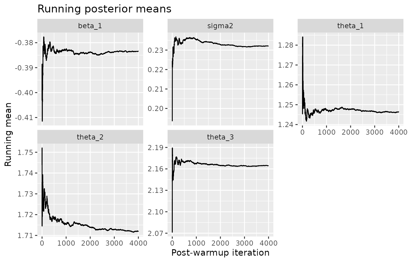
If the running means stabilize, that is usually a good sign that Monte Carlo error is shrinking.

Simple numerical diagnostics

ess_simple <- function(x, max_lag = 100) {
  acf_vals <- stats::acf(
    x,
    lag.max = min(max_lag, length(x) - 1),
    plot = FALSE
  )$acf[-1]

  positive_acf <- acf_vals[acf_vals > 0]

  if (length(positive_acf) == 0) {
    return(length(x))
  }

  tau <- 1 + 2 * sum(positive_acf)
  min(length(x), length(x) / tau)
}

diagnostics <- data.frame(
  parameter = colnames(fit$draws),
  mean = colMeans(fit$draws),
  sd = apply(fit$draws, 2, sd),
  lag1_acf = apply(fit$draws, 2, function(x) stats::acf(x, lag.max = 1, plot = FALSE)$acf[2]),
  ess = apply(fit$draws, 2, ess_simple),
  mcse = mapply(function(s, e) s / sqrt(e), apply(fit$draws, 2, sd), apply(fit$draws, 2, ess_simple)),
  row.names = NULL
)

diagnostics
#>   parameter       mean         sd   lag1_acf      ess         mcse
#> 1   theta_1  1.2463566 0.06462694 0.07715308 1670.518 0.0015812045
#> 2   theta_2  1.7120960 0.06780666 0.17671633 1401.528 0.0018112211
#> 3   theta_3  2.1643972 0.07989574 0.36812889 1153.227 0.0023526984
#> 4    beta_1 -0.3834375 0.04700082 0.33138567 1187.507 0.0013639152
#> 5    sigma2  0.2321148 0.03015053 0.33885848 1020.186 0.0009439638

Lower autocorrelation and higher effective sample size are usually preferable.

Repeat the fit with different seeds

fit_seeds <- lapply(c(6841, 7313, 8129), function(seed) {
  exnex_surv(
    Surv(time, event) ~ group + age_std,
    data = sim_data,
    iter = 3000,
    warmup = 1000,
    chains = 2,
    parallel_chains = 2,
    seed = seed
  )
})

posterior_means_by_run <- do.call(
  rbind,
  lapply(fit_seeds, function(x) {
    s <- summary(x)
    stats::setNames(s$mean, s$parameter)
  })
)

posterior_means_by_run
#>       theta_1  theta_2  theta_3     beta_1    sigma2
#> [1,] 1.246357 1.712096 2.164397 -0.3834375 0.2321148
#> [2,] 1.243725 1.711442 2.161590 -0.3829936 0.2310015
#> [3,] 1.245225 1.710733 2.162179 -0.3825527 0.2325135
apply(posterior_means_by_run, 2, sd)
#>      theta_1      theta_2      theta_3       beta_1       sigma2 
#> 0.0013202950 0.0006818794 0.0014800891 0.0004424412 0.0007836361

If posterior means are very similar across runs, that supports stability.

Interpretation

These diagnostics are practical checks, not formal proofs of convergence. Still, when traceplots look stable, running means flatten out, and repeated runs give similar posterior summaries, the fit is usually behaving reasonably well.