Tools for Experimenters

Beyond fitting, exnexSurv provides a small set of inference and model-selection utilities that operate directly on the posterior draws already stored in a fitted exnex_surv object. This vignette walks through each of them using a small simulated example.

A quick simulated example

We first generate a basket-trial dataset with simulate_data(). By default it creates K = 9 baskets with n = 30 patients each, a single covariate, and lets us flag some baskets as “resistant” (their location is shifted away from the healthy population) — exactly the situation the EXNEX model is designed to handle.

library(exnexSurv)
library(survival)

set.seed(42)
d <- simulate_data(
  n = 20,
  beta = 0.5,
  sigma = 1.1,
  outlier_baskets = c(2, 8),
  resist_delta = -1.0,
  censoring_rate = 0.3,
  seed = 1
)

head(d)
#>         time event group         x1
#> 1 0.18911694     0     1 -0.3053884
#> 2 0.09337518     0     1  1.5117812
#> 3 0.76338340     0     1  0.3898432
#> 4 0.29834303     1     1 -0.6212406
#> 5 0.74983093     1     1 -2.2146999
#> 6 0.42299553     1     1  1.1249309

The dataset stores the true generating parameters as attributes:

attr(d, "true_theta")
#> [1] -0.09396807 -0.97245350 -0.12534429  0.23929212  0.04942617 -0.12307026
#> [7]  0.07311436 -0.88925129  0.08636720
attr(d, "true_beta")
#> [1] 0.5
attr(d, "true_sigma")
#> [1] 1.1

Now fit the model. We keep the chain short so the vignette builds quickly; for real work use more iterations and multiple chains.

fit <- exnex_surv(
  Surv(time, event) ~ group + x1,
  data = d,
  iter = 2000,
  warmup = 1000,
  chains = 2,
  seed = 7
)
print(fit, show_trace = FALSE)
#> <exnex_surv model>
#> Draws: 2000 total post-warmup samples
#>        1000 post-warmup samples per chain
#> Groups: 9 | Covariates: 1 
#> MCMC: iter = 2000 , warmup = 1000 , chains = 2 
#> 
#>  parameter        mean        sd        q05         q50        q95
#>    theta_1  0.11669485 0.3069765 -0.3559653  0.10164526  0.6594590
#>    theta_2 -0.93329406 0.2705633 -1.3614140 -0.94103137 -0.4745091
#>    theta_3 -0.39262307 0.3118125 -0.8972846 -0.39517207  0.1279407
#>    theta_4  0.32611057 0.3096740 -0.1786917  0.31792317  0.8508286
#>    theta_5 -0.06263464 0.2780822 -0.5129246 -0.07036695  0.3991122
#>    theta_6  0.18591764 0.3207427 -0.3435120  0.18593333  0.7207398
#>    theta_7  0.22624399 0.3367305 -0.3136029  0.22118365  0.7945553
#>    theta_8 -0.81203876 0.2875932 -1.2800821 -0.81498863 -0.3578141
#>    theta_9 -0.01260007 0.3443596 -0.5723189 -0.02049141  0.5682546
#>     beta_1  0.58664689 0.1243464  0.3808375  0.58879860  0.7866019
#>     sigma2  1.45675160 0.2336813  1.1254281  1.43078082  1.8681451

Survival curves

survival_curves() evaluates the posterior survival function $S(t) = \Pr(T > t)$ on a time grid, returning a data frame with the posterior median and a credible band:

curves <- survival_curves(fit)
#> Warning: More than one group present (1, 2, 3, 4, 5, 6, 7, 8, 9). Only the
#> first group '1' is used. Supply `newdata` with a `group` column to evaluate
#> specific groups.
head(curves)
#>         time    median     lower     upper group
#> 1 0.00000000 1.0000000 1.0000000 1.0000000     1
#> 2 0.02167666 0.9995105 0.9961272 0.9999611     1
#> 3 0.04335333 0.9966598 0.9837442 0.9995352     1
#> 4 0.06502999 0.9911528 0.9664658 0.9983715     1
#> 5 0.08670666 0.9834503 0.9459817 0.9963951     1
#> 6 0.10838332 0.9741849 0.9252277 0.9936357     1

plot.survival_exnex() draws the curves (requires ggplot2):

plot(curves)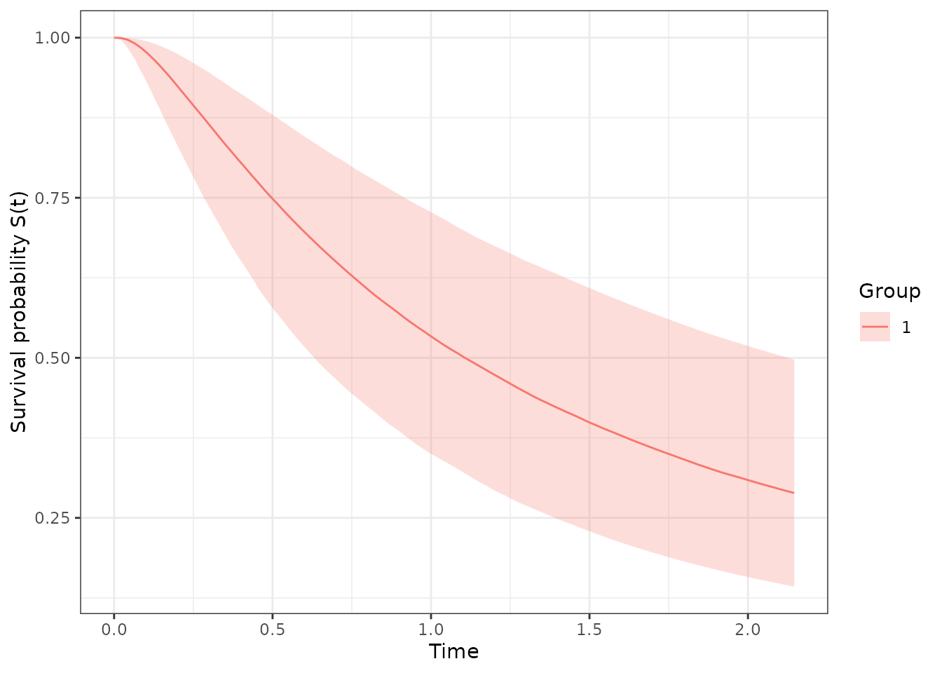

By default a single curve is produced with covariates fixed at zero. Passing newdata evaluates one row per subject with its own covariate values and group:

nd <- data.frame(group = d$group[1:3], x1 = c(0, 0.2, -0.1))
curves_nd <- survival_curves(fit, newdata = nd)
table(curves_nd$group)
#> 
#>   1   2   3 
#> 100 100 100

Posterior median survival time

For the log-normal AFT model the median survival time of a linear predictor $\eta$ is simply $\exp(\eta)$. median_survival() reports its posterior quantiles with credible intervals:

median_survival(fit)
#> Warning: More than one group present (1, 2, 3, 4, 5, 6, 7, 8, 9). Only the
#> first group '1' is used. Supply `newdata` with a `group` column to evaluate
#> specific groups.
#>     group   median     lower    upper
#> 50%     1 1.106991 0.6315226 2.126547

Restricted mean survival time (RMST)

rmst() computes $\mathrm{RMST}(t_{max}) = \int_0^{t_{max}} S(t)\,dt$ for each posterior draw and summarises the distribution:

rmst(fit, tmax = 10)
#> Warning: More than one group present (1, 2, 3, 4, 5, 6, 7, 8, 9). Only the
#> first group '1' is used. Supply `newdata` with a `group` column to evaluate
#> specific groups.
#>     group     rmst    lower    upper
#> 50%     1 2.000315 1.177118 3.416444

Model comparison with WAIC

compute_waic() evaluates the pointwise log-likelihood of the observed data (here the censoring contribution is handled explicitly), giving WAIC, its standard error, the log pointwise predictive density (lpd) and the penalty p_waic:

w <- compute_waic(fit)
str(w[c("waic", "se_elpd_waic", "lpd", "p_waic", "elpd_waic")])
#> List of 5
#>  $ waic        : num 185
#>  $ se_elpd_waic: num 7.61
#>  $ lpd         : num -83.2
#>  $ p_waic      : num 9.54
#>  $ elpd_waic   : num -92.7

compare_waic() contrasts several fits (e.g. a full model vs. a group-only model) and returns them ordered by ascending WAIC:

fit_group <- exnex_surv(
  Surv(time, event) ~ group,
  data = d,
  iter = 2000, warmup = 1000, chains = 2, seed = 7
)

compare_waic(without_covariate = fit_group, with_covariate = fit)
#>               model   waic se_elpd_waic       lpd   p_waic elpd_waic
#> 1    with_covariate 185.48         7.61 -83.19976 9.538642  -92.7384
#> 2 without_covariate 208.14         6.64 -95.30619 8.762752 -104.0689

Probability that one group beats another

probability_superiority() estimates $\Pr(\mathrm{summ}_a > \mathrm{summ}_b)$ draw-by-draw for one of three summaries: median survival, survival probability at a fixed time, or RMST.

# Median survival
probability_superiority(fit, a = 1, b = 3, function_of = "median")
#> $prob
#> [1] 0.881
#> 
#> $summary
#> [1] "median"
#> 
#> $groups
#> a b 
#> 1 3

# Survival probability at t = 3
probability_superiority(fit, a = 1, b = 2, function_of = "survival", times = 3)
#> $prob
#> [1] 0.9955
#> 
#> $summary
#> [1] "survival"
#> 
#> $groups
#> a b 
#> 1 2

# RMST up to t = 10
probability_superiority(fit, a = 1, b = 2, function_of = "rmst", tmax = 10)
#> $prob
#> [1] 0.9955
#> 
#> $summary
#> [1] "rmst"
#> 
#> $groups
#> a b 
#> 1 2

In this example baskets 1 and 3 are both healthy (only 2 and 8 are resistant), so probability_superiority() comparing them has no reason to prefer one over the other and returns a probability close to 0.5. The exact numbers will vary with the simulated data and the MCMC run.