Getting Started with exnexSurv

Overview

exnexSurv fits Bayesian EXNEX survival models for right-censored log-normal data. The current interface supports:

a formula interface,
an x/y interface,
subgroup effects,
optional covariates,
posterior draws for theta_j, beta, and sigma2.

Simulate a simple dataset

library(exnexSurv)
library(survival)

simulate_surv_data <- function(
  theta,
  sigma2,
  beta = NULL,
  n_per_group = 50,
  censor_min = 4,
  censor_max = 12,
  seed = NULL
) {
  if (!is.null(seed)) {
    set.seed(seed)
  }

  groups <- rep(seq_along(theta), each = n_per_group)
  age_std <- rnorm(length(groups), mean = 0, sd = 1)
  mean_log_time <- rep(theta, each = n_per_group)

  if (!is.null(beta)) {
    mean_log_time <- mean_log_time + beta * age_std
  }

  log_time <- rnorm(length(groups), mean = mean_log_time, sd = sqrt(sigma2))
  true_time <- exp(log_time)
  censor_time <- runif(length(groups), min = censor_min, max = censor_max)

  data.frame(
    time = pmin(true_time, censor_time),
    event = as.integer(true_time <= censor_time),
    group = factor(groups),
    age_std = age_std
  )
}

sim_data <- simulate_surv_data(
  theta = c(1.1, 1.6, 2.0),
  sigma2 = 0.25,
  beta = -0.30,
  n_per_group = 50,
  seed = 6421
)

head(sim_data)
#>       time event group    age_std
#> 1 3.339087     1     1  0.6071040
#> 2 3.330683     1     1 -1.1474496
#> 3 2.469950     1     1 -0.5987154
#> 4 4.277826     1     1 -1.6561367
#> 5 2.422691     1     1  0.8235441
#> 6 2.831290     1     1  0.5040783
mean(sim_data$event)
#> [1] 0.7866667

Fit the model with a formula

fit_formula <- exnex_surv(
  Surv(time, event) ~ group + age_std,
  data = sim_data,
  iter = 1200,
  warmup = 400,
  chains = 1,
  seed = 6421
)

print(fit_formula, show_trace = FALSE)
#> <exnex_surv model>
#> Draws: 800 total post-warmup samples
#>        800 post-warmup samples per chain
#> Groups: 3 | Covariates: 1 
#> MCMC: iter = 1200 , warmup = 400 , chains = 1 
#> 
#>  parameter       mean         sd        q05        q50        q95
#>    theta_1  0.9861505 0.06849275  0.8788059  0.9862140  1.0958766
#>    theta_2  1.5326028 0.07082872  1.4121900  1.5318814  1.6524219
#>    theta_3  1.9841454 0.07555761  1.8632978  1.9833107  2.1082712
#>     beta_1 -0.3075793 0.04281121 -0.3797194 -0.3074616 -0.2362734
#>     sigma2  0.2347691 0.03216346  0.1856459  0.2331866  0.2883242
summary(fit_formula)
#>   parameter       mean         sd        q05        q50        q95
#> 1   theta_1  0.9861505 0.06849275  0.8788059  0.9862140  1.0958766
#> 2   theta_2  1.5326028 0.07082872  1.4121900  1.5318814  1.6524219
#> 3   theta_3  1.9841454 0.07555761  1.8632978  1.9833107  2.1082712
#> 4    beta_1 -0.3075793 0.04281121 -0.3797194 -0.3074616 -0.2362734
#> 5    sigma2  0.2347691 0.03216346  0.1856459  0.2331866  0.2883242

The fitted object stores the processed data, posterior draws, and MCMC settings. You can inspect the model structure with the usual S3 methods.

Run multiple chains in parallel

fit_parallel <- exnex_surv(
  Surv(time, event) ~ group + age_std,
  data = sim_data,
  iter = 1200,
  warmup = 400,
  chains = 2,
  parallel_chains = 2,
  seed = 6421
)

print(fit_parallel, show_trace = FALSE)
#> <exnex_surv model>
#> Draws: 1600 total post-warmup samples
#>        800 post-warmup samples per chain
#> Groups: 3 | Covariates: 1 
#> MCMC: iter = 1200 , warmup = 400 , chains = 2 
#> 
#>  parameter       mean         sd        q05        q50        q95
#>    theta_1  0.9870040 0.06958675  0.8748666  0.9858982  1.0979172
#>    theta_2  1.5334538 0.07136513  1.4126375  1.5335034  1.6516964
#>    theta_3  1.9815311 0.07540195  1.8590322  1.9798331  2.1025855
#>     beta_1 -0.3047351 0.04333179 -0.3782277 -0.3047538 -0.2341006
#>     sigma2  0.2337765 0.03210020  0.1862492  0.2316788  0.2892194
plot(
  fit_parallel,
  parameters = c("theta_1", "theta_2", "theta_3", "beta_1", "sigma2"),
  ask = FALSE
)

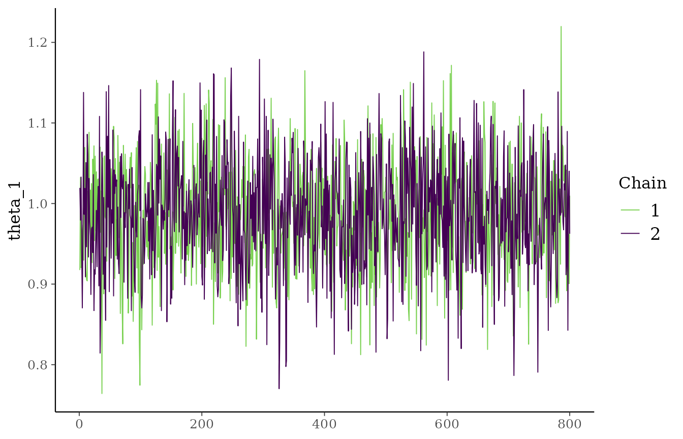
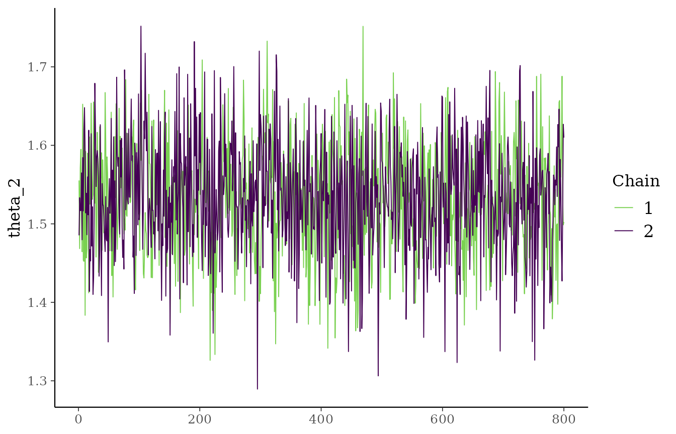
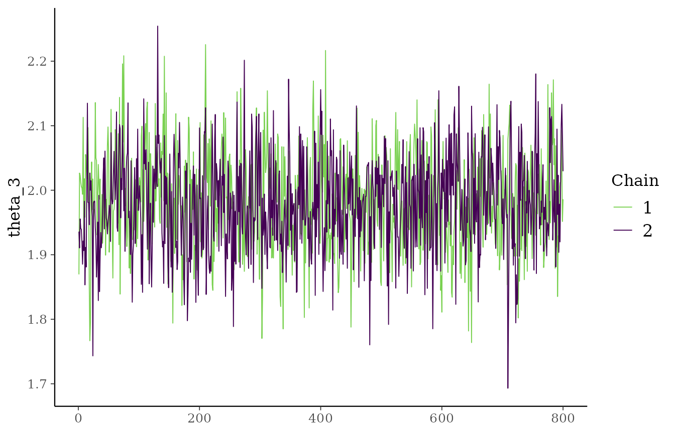
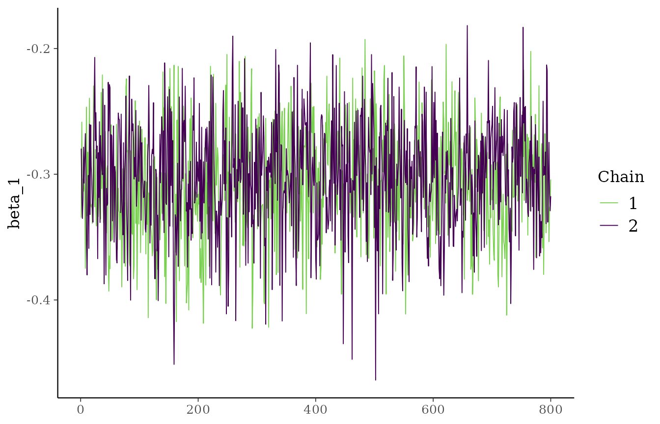
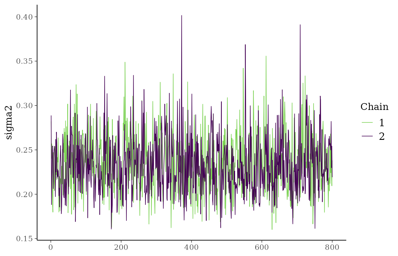
When parallel_chains is greater than 1, the chains are evaluated concurrently by R and the traceplots show all chains in the same panel for each parameter.

If you do not want to use all available workers, set parallel_chains smaller than chains. For example, chains = 4 and parallel_chains = 2 runs four independent chains while evaluating two at a time.

The fitted object stores the combined post-warmup draws from all chains in one table. Because each chain contributes the same number of post-warmup samples, the total number of rows is (iter - warmup) * chains.

str(fit_formula$data)
#> List of 9
#>  $ time        : num [1:150] 3.34 3.33 2.47 4.28 2.42 ...
#>  $ event       : num [1:150] 1 1 1 1 1 1 1 1 1 1 ...
#>  $ group       : num [1:150] 1 1 1 1 1 1 1 1 1 1 ...
#>  $ X           : num [1:150, 1] 0.607 -1.147 -0.599 -1.656 0.824 ...
#>   ..- attr(*, "dimnames")=List of 2
#>   .. ..$ : NULL
#>   .. ..$ : chr "age_std"
#>  $ n           : int 150
#>  $ n_groups    : num 3
#>  $ n_covariates: int 1
#>  $ cov_names   : chr "age_std"
#>  $ chain_seeds : int 979729617
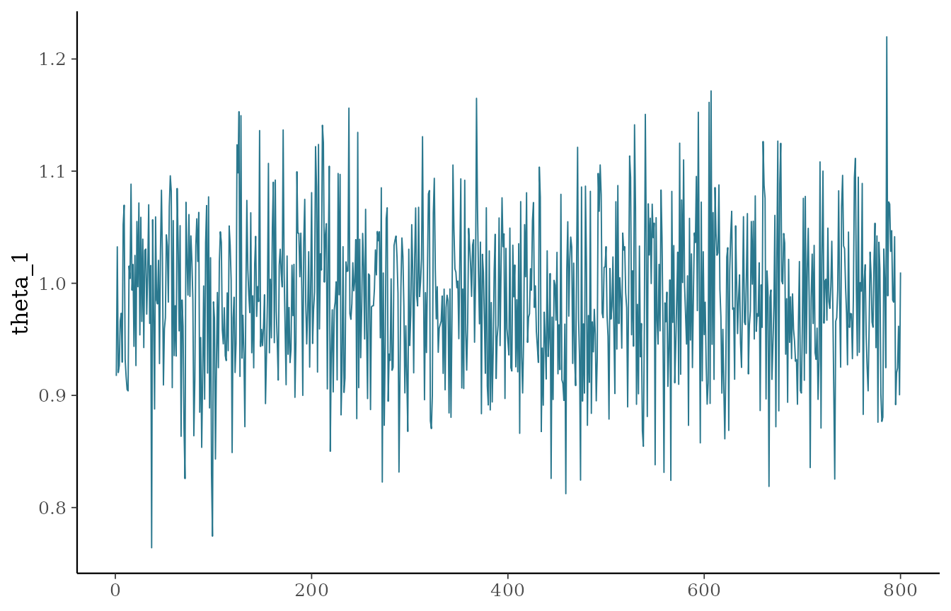
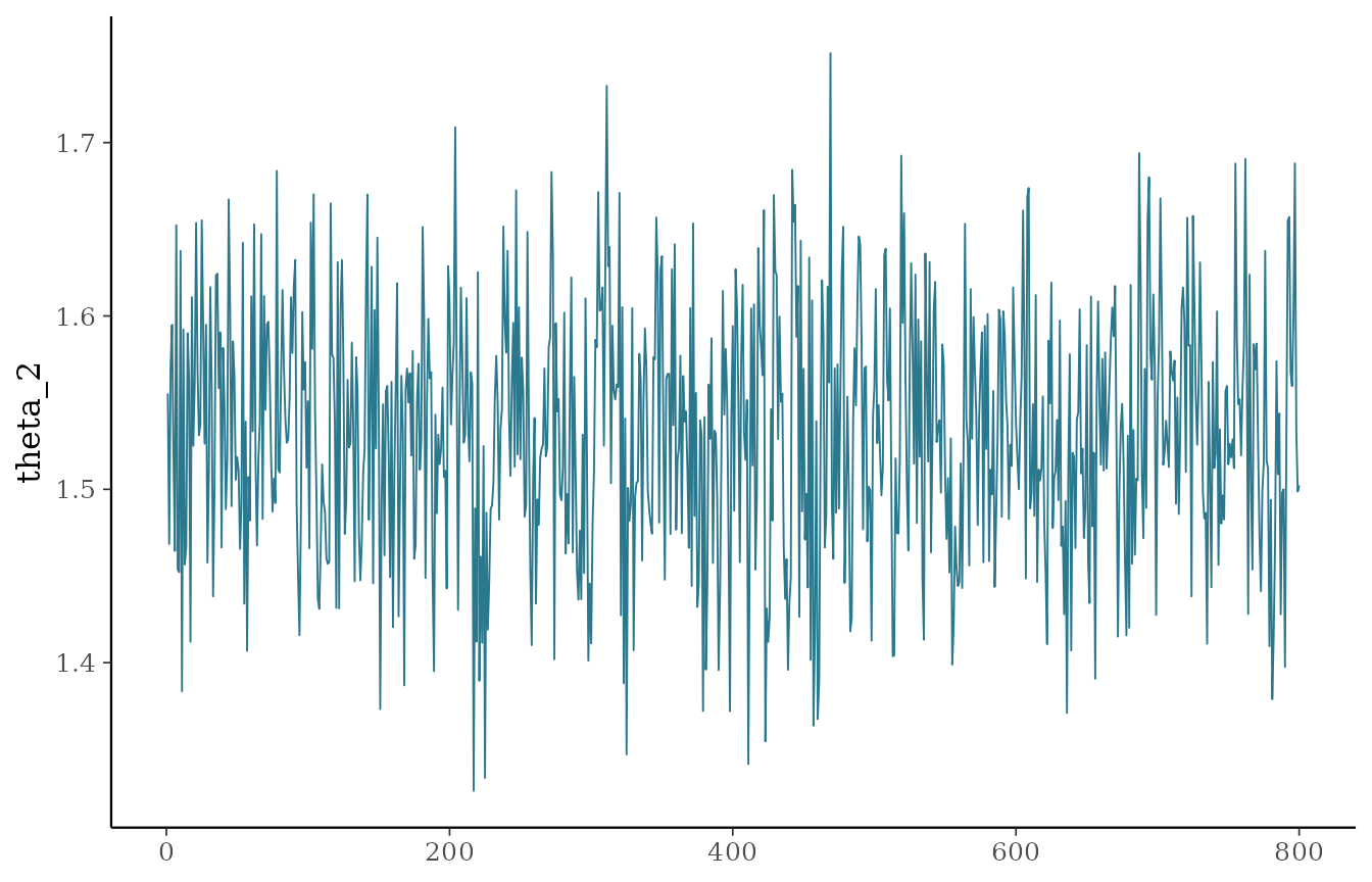
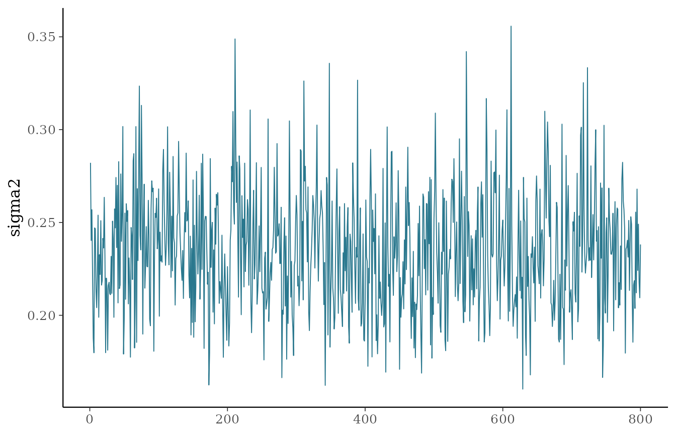
plot(
  fit_formula,
  parameters = c("theta_1", "theta_2", "sigma2"),
  ask = FALSE
)

Fit the model with `x` and `y`

fit_xy <- exnex_surv(
  x = sim_data[c("group", "age_std")],
  y = Surv(sim_data$time, sim_data$event),
  iter = 1200,
  warmup = 400,
  chains = 1,
  seed = 6421
)

summary(fit_xy)
#>   parameter       mean         sd        q05        q50        q95
#> 1   theta_1  0.9861505 0.06849275  0.8788059  0.9862140  1.0958766
#> 2   theta_2  1.5326028 0.07082872  1.4121900  1.5318814  1.6524219
#> 3   theta_3  1.9841454 0.07555761  1.8632978  1.9833107  2.1082712
#> 4    beta_1 -0.3075793 0.04281121 -0.3797194 -0.3074616 -0.2362734
#> 5    sigma2  0.2347691 0.03216346  0.1856459  0.2331866  0.2883242
all.equal(fit_formula$draws, fit_xy$draws)
#> [1] TRUE

This is useful if predictors and outcomes are prepared separately.

Fit a model without covariates

If the model only contains the subgroup variable, no beta terms are estimated.

fit_no_cov <- exnex_surv(
  Surv(time, event) ~ group,
  data = sim_data,
  iter = 1200,
  warmup = 400,
  chains = 1,
  seed = 6421
)

summary(fit_no_cov)
#>   parameter      mean         sd       q05       q50       q95
#> 1   theta_1 0.9610428 0.07667525 0.8240873 0.9646688 1.0782239
#> 2   theta_2 1.5114113 0.08415282 1.3716898 1.5122529 1.6479938
#> 3   theta_3 1.9543858 0.08866337 1.8051221 1.9554501 2.0994038
#> 4    sigma2 0.3194790 0.04445914 0.2526799 0.3156426 0.4000848
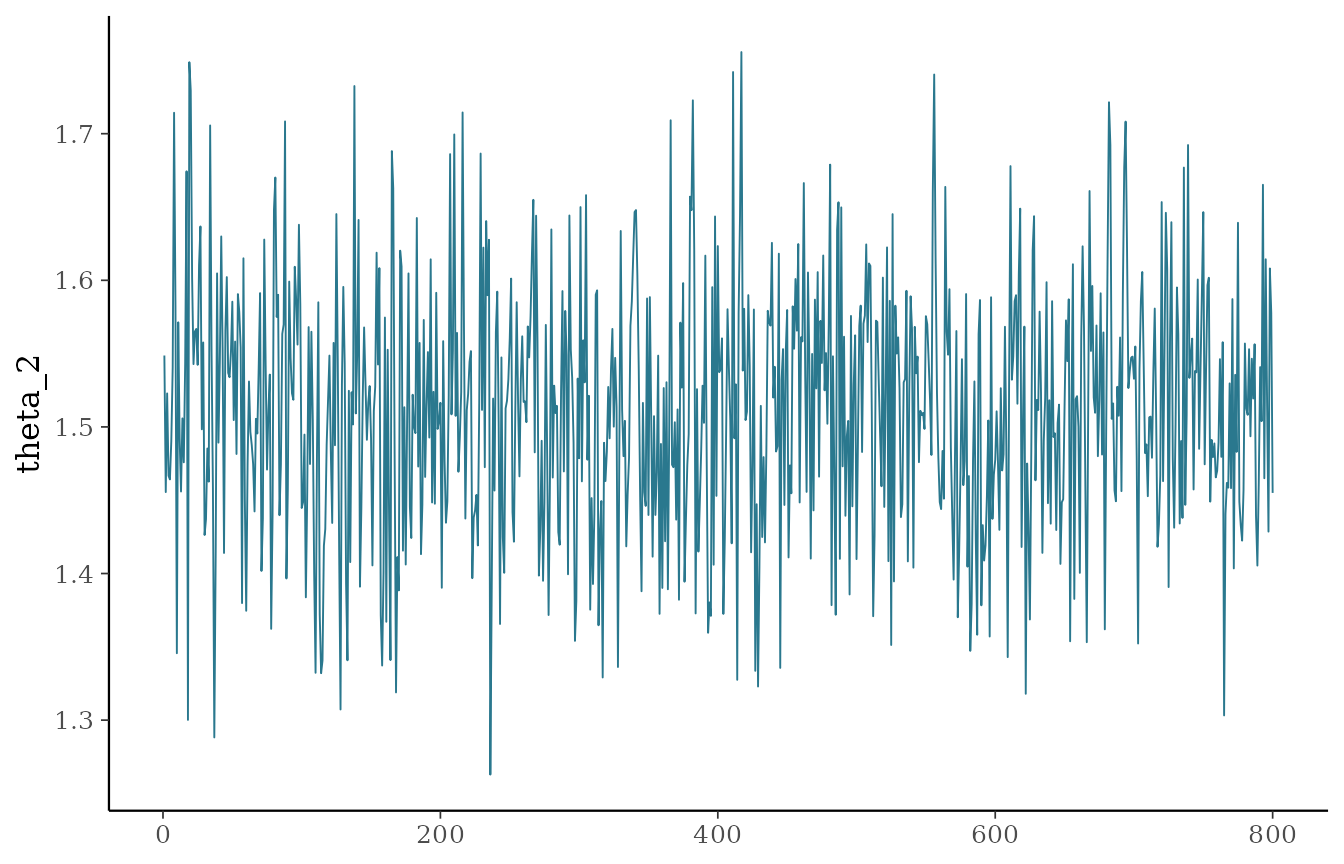
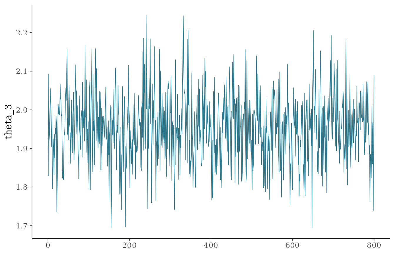
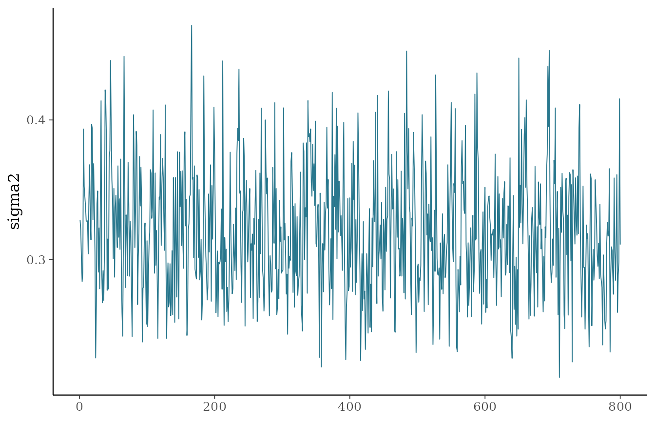
plot(fit_no_cov, ask = FALSE)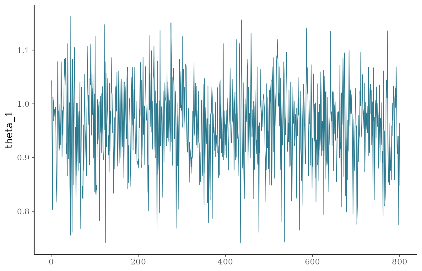

Basic posterior summaries

summary(fit_formula)
#>   parameter       mean         sd        q05        q50        q95
#> 1   theta_1  0.9861505 0.06849275  0.8788059  0.9862140  1.0958766
#> 2   theta_2  1.5326028 0.07082872  1.4121900  1.5318814  1.6524219
#> 3   theta_3  1.9841454 0.07555761  1.8632978  1.9833107  2.1082712
#> 4    beta_1 -0.3075793 0.04281121 -0.3797194 -0.3074616 -0.2362734
#> 5    sigma2  0.2347691 0.03216346  0.1856459  0.2331866  0.2883242

Inspecting the resolved priors

Whatever you pass to priors, the fitted object records the exact hyperparameters the sampler used, with defaults merged into the fields you did not supply. This is useful to confirm your customization was applied and to reproduce a fit.

fit_formula$resolved_priors
#> $a_sigma
#> [1] 2
#> 
#> $b_sigma
#> [1] 2
#> 
#> $a_tau
#> [1] 2
#> 
#> $b_tau
#> [1] 2
#> 
#> $p_mix
#> [1] 0.5
#> 
#> $m_mu
#> [1] 0
#> 
#> $v_mu
#> [1] 10000
#> 
#> $m_nex
#> [1] 0
#> 
#> $v_nex
#> [1] 10000
#> 
#> $v_beta
#> [1] 10000

To customize a prior, pass a named list to priors; for example, priors = list(p_mix = 0.7, a_tau = 3, b_tau = 3). The fields p_mix, m_nex, and v_nex also accept a vector of length equal to the number of baskets, assigning one value per basket. See the vignette The EXNEX Model, Priors, and Data Augmentation for the full list of hyperparameters and how to set them.

Notes

The current implementation supports multiple chains, including R-level parallel execution through parallel_chains. For a more careful convergence check, fit more than one chain and compare the traceplots and posterior summaries across chains.