The EXNEX Model, Priors, and Data Augmentation • exnexSurv

Introduction

Basket trials enroll patients into several small groups (baskets), often defined by a biomarker, tumor histology, or cancer type, that are studied under a common protocol. Because each basket typically contains only a handful of patients, separately estimating an effect in every basket is imprecise, while pooling all patients into a single estimate ignores real differences between baskets. Borrowing of information across baskets strikes a middle ground: baskets that look alike share strength, while baskets that disagree with the majority are allowed to stand apart.

The EXNEX (Exchangeable–Non-Exchangeable) framework extends the standard exchangeable hierarchical model by attaching a latent indicator to every basket that selects whether its effect is drawn from a shared exchangeable component or from a basket-specific non-exchangeable prior [@neuenschwander2016]. exnexSurv implements EXNEX for right-censored, log-normal survival data using a data-augmented Gibbs sampler written in C++ via Rcpp and RcppArmadillo [@eddelbuettel2011rcpp; @sanderson2016armadillo].

This vignette explains the model, the priors and how to customize them, the data augmentation mechanism that makes the sampler exact and fast, the systematic Gibbs scan, and what the fitted object contains. A short worked example illustrates shrinkage and prior customization. The statistical methodology is described in detail in the companion paper (Ney, 2026); the performance numbers quoted in the last section are taken from it.

The model

For patient $i$ let $T_i$ denote the true event time, $C_i$ the censoring time, $Y_i=\min(T_i,C_i)$ the observed follow-up time, $\delta_i=\mathbb 1(T_i\le C_i)$ the event indicator, $g[i]\in\{1,\ldots,K\}$ the basket assignment, and $X_i$ a $P$ -vector of covariates. The complete model is

$\begin{aligned} \log T_i &= \theta_{g[i]}+X_i^{\mathsf T}\beta+\varepsilon_i, &&\varepsilon_i\sim\mathcal N(0,\sigma^2),\\ \theta_j\mid Z_j &\sim Z_j\,\mathcal N(\mu,\tau^2)+(1-Z_j)\,\mathcal N(m_{0j},v_{0j}), &&Z_j\sim\mathrm{Bern}(p_{\mathrm{exch},j}), \end{aligned}$

with $p_{\mathrm{exch},j}=0.5$ , $m_{0j}=0$ , $v_{0j}=10^4$ by default, and the diffuse hyperpriors

$\mu\sim\mathcal N(0,10^4),\qquad \tau^2\sim\mathcal{IG}(2,2),\qquad \sigma^2\sim\mathcal{IG}(2,2).$

Here $\theta_j$ is the covariate-adjusted location of log survival in basket $j$ . Because the model is log-normal, $\exp(\theta_j-\theta_{j'})$ is the ratio of conditional median survival times between baskets $j$ and $j'$ . Notation is summarized in Table .

Notation.
Symbol	Meaning
$T_i$ , $C_i$ , $Y_i$	true event time, censoring time, observed time
$\delta_i$	event indicator (1 = observed event, 0 = censored)
$g[i]$ , $K$	basket index of patient $i$ ; number of baskets
$X_i$ , $P$	covariate vector; number of covariates
$\theta_j$	log-location effect of basket $j$ (target of inference)
$\beta$	regression coefficients
$\sigma^2$	common residual variance
$\mu$ , $\tau^2$	exchangeable mean and between-basket variance
$Z_j$	latent indicator: $1$ = exchangeable, $0$ = non-exchangeable
$p_{\mathrm{exch},j}$	prior probability that basket $j$ is exchangeable
$m_{0j}$ , $v_{0j}$	prior mean and variance of the non-exchangeable component

The residual variance $\sigma^2$ is assumed common across baskets. This is a deliberate choice: the smallest baskets contain roughly five to fifteen patients and even fewer observed events, so basket-specific residual variances would be weakly identified and highly sensitive to the prior. Clinically relevant between-basket heterogeneity is instead represented through the location effects $\theta_j$ and the between-basket variance $\tau^2$ . This restriction is a limitation of the model and is examined empirically in the companion paper.

Priors and how to customize them

Normal priors are parameterized by variance. A value of $10^4$ corresponds to a prior standard deviation of $100$ on the log-time scale, which we treat as an extremely diffuse reference default rather than a clinically elicited prior. The inverse-Gamma priors use the shape–rate parameterization: $X\sim\mathcal{IG}(a,b)$ has density $\propto x^{-a-1}e^{-b/x}$ , with mean $b/(a-1)$ for $a>1$ .

The table below lists every prior hyperparameter, its default, and its role.

`priors` field	Role	Default
`a_sigma`, `b_sigma`	shape, rate of $\sigma^2$ prior $\mathcal{IG}$	`2`, `2`
`a_tau`, `b_tau`	shape, rate of $\tau^2$ prior $\mathcal{IG}$	`2`, `2`
`p_mix`	mixture weight $p_{\mathrm{exch},j}$	`0.5`
`m_mu`, `v_mu`	prior mean, variance of $\mu$	`0`, `1e4`
`m_nex`, `v_nex`	prior mean, variance of non-exchangeable component	`0`, `1e4`
`v_beta`	variance of the regression-coefficient prior (precision $1/v_{\beta}I$ )	`1e4`

All fields are optional: absent fields keep the defaults and unknown fields are ignored. Customize a prior by passing a named list to exnex_surv():

fit <- exnex_surv(
  Surv(time, event) ~ group,
  data = d,
  priors = list(
    p_mix  = 0.7,
    v_nex  = 10,
    a_tau  = 3,
    b_tau  = 3,
    v_beta = 10
  )
)

The fields p_mix, m_nex, and v_nex each accept either a scalar (replicated across all baskets) or a numeric vector of length $K$ with one value per basket, matching the basket-specific notation $p_{\mathrm{exch},j}$ , $m_{0j}$ , $v_{0j}$ of the model. This makes it possible, for example, to give some baskets a strong non-exchangeable prior while leaving the others exchangeable. The sampler validates the inputs: p_mix must lie strictly between 0 and 1 for every basket, variances must be positive, and a supplied vector must have exactly $K$ elements.

After a fit, fit$resolved_priors reports the hyperparameters that were actually used (defaults merged with any overrides), which is a convenient way to confirm your customization was applied:

library(exnexSurv)
library(survival)
library(ggplot2)

simulate_basket_data <- function(
  theta,
  sigma = 1.2,
  beta = c(0.8, -0.5),
  group_sizes = c(30, 24, 20, 16, 14, 11, 8, 7, 5),
  target_cens = 0.30,
  seed = 1
) {
  set.seed(seed)
  K <- length(theta)
  group <- rep(seq_len(K), times = group_sizes)
  n <- length(group)
  X1 <- rnorm(n)
  X2 <- rnorm(n)
  eta <- theta[group] + X1 * beta[1] + X2 * beta[2]
  log_time <- eta + rnorm(n, 0, sigma)
  true_time <- exp(log_time)
  censor_fun <- function(c) mean(true_time > c) - target_cens
  censor_time <- uniroot(censor_fun, c(min(true_time), max(true_time)))$root
  data.frame(
    time = pmin(true_time, censor_time),
    event = as.integer(true_time <= censor_time),
    group = factor(group),
    X1 = X1,
    X2 = X2
  )
}

theta_true <- c(1.5, 1.4, 1.6, 1.45, 1.55, 1.5, -0.4, -0.6, -0.5)
d <- simulate_basket_data(theta_true, seed = 1)

# small, quick fit just to inspect resolved_priors
quick <- exnex_surv(
  Surv(time, event) ~ group + X1 + X2,
  data = d,
  priors = list(p_mix = 0.7, v_nex = 10),
  iter = 400, warmup = 200, chains = 1
)
print(quick$resolved_priors)
#> $a_sigma
#> [1] 2
#> 
#> $b_sigma
#> [1] 2
#> 
#> $a_tau
#> [1] 2
#> 
#> $b_tau
#> [1] 2
#> 
#> $p_mix
#> [1] 0.7
#> 
#> $m_mu
#> [1] 0
#> 
#> $v_mu
#> [1] 10000
#> 
#> $m_nex
#> [1] 0
#> 
#> $v_nex
#> [1] 10
#> 
#> $v_beta
#> [1] 10000

The printed list shows the customized p_mix and v_nex alongside the default values for the fields you did not touch.

Model variants

The EXNEX hierarchy is flexible enough to recover two familiar alternatives, which are useful as references for comparison:

Setting	Description	How to approximate
EXNEX (default)	selective borrowing via latent $Z_j$	the default prior
EX (full exchangeability)	all $\theta_j$ share $\mathcal N(\mu,\tau^2)$	`p_mix = 0.9999999`
No pooling	independent basket effects	`p_mix = 1e-6`, large `v_nex`

Because the mixture weight is validated to be strictly between 0 and 1, a fully exchangeable model is approximated with p_mix extremely close to 1, and a no-pooling model with p_mix extremely close to 0 together with a diffuse v_nex. Complete pooling (a single shared intercept) is not directly expressible in the current formula interface, which requires at least one right-hand-side variable to identify the group; it can be emulated by fitting a single basket.

Data augmentation

The sampler is best understood as a missing-data construction. The censored event times are, literally, missing observations: for a censored patient we know only that $T_i>C_i$ , and if we could observe the true $T_i$ the likelihood would be a complete-data Gaussian regression. Data augmentation [@tanner1987calculation] treats the unobserved quantities as additional unknowns and alternates between imputing them from their conditional distribution and updating the model parameters.

Why is the observed-data likelihood inconvenient? For an observed event at time $Y_i$ , the log-normal density contributes a Gaussian term in $\log Y_i$ , but a censored observation contributes only the survival probability

$S(Y_i)=1-\Phi\!\left(\frac{\log Y_i-\eta_i}{\sigma}\right),\qquad \eta_i=\theta_{g[i]}+X_i^{\mathsf T}\beta.$

The standard Normal CDF $\Phi$ has no antiderivative in elementary functions; equivalently, the censored contribution is an integral of the complete-data Gaussian likelihood over the region $\log T_i>\log Y_i$ . This integral cannot be collapsed into a conjugate update and would have to be evaluated numerically at every parameter value. Data augmentation sidesteps the integral entirely: instead of evaluating $S(Y_i)$ , the sampler draws the missing log-time from its conditional distribution, after which only the complete-data Gaussian likelihood remains.

Conditional on the parameters, a censored log-time follows a truncated Normal,

$z_i\mid\delta_i=0,\ \cdot\ \sim \mathcal{TN}_{(\ell_i,\infty)}(\eta_i,\sigma^2),\qquad \ell_i=\log Y_i,$

whose density is the Gaussian density restricted to the censored region and renormalized. Draws are generated by inverse-CDF transformation evaluated entirely in log space, which remains numerically stable when the censoring threshold is far in the upper tail and needs no accept–reject step. After every censored $z_i$ is imputed, the model is an ordinary Gaussian linear regression and every parameter block has a known full conditional.

The joint posterior kernel makes the conjugacy explicit:

$\begin{aligned} p(\theta,Z,\mu,\tau^2,\beta,\sigma^2\mid z)&\propto (\sigma^2)^{-N/2}\exp\!\left\{-\frac{1}{2\sigma^2}\sum_{i=1}^{N}(z_i-\eta_i)^2\right\}\\ &\quad\times\prod_{j=1}^{K} \left[p_{\mathrm{exch},j}\,\varphi(\theta_j;\mu,\tau^2)\right]^{Z_j} \left[(1-p_{\mathrm{exch},j})\,\varphi(\theta_j;m_{0j},v_{0j})\right]^{1-Z_j}\\ &\quad\times p(\mu)\,p(\tau^2)\,p(\sigma^2), \end{aligned}$

where $\varphi(\cdot;m,v)$ is the Normal density with mean $m$ and variance $v$ . Every factor is a known kernel, which is what makes the systematic scan of the sampler exact. It also explains a geometric advantage over Hamiltonian samplers on the observed-data posterior: marginalizing out the discrete indicators $Z_j$ leaves a mixture of up to $2^K$ Normal components in the basket-effect space, a multimodal geometry that is hard for NUTS to navigate. The augmented sampler keeps the indicators explicit and updates them one at a time, so it never has to traverse that mixture landscape.

The Gibbs sampler

Each iteration performs the following systematic scan.

# 1. Impute censored log-event times z_i ~ TN(log Y_i, Inf)(eta_i, sigma^2)
# 2. Update residual variance sigma^2
# 3. Update regression coefficients beta
# 4. Update basket effects theta_j ~ N(m_j, V_j)
# 5. Update mixture indicators Z_j ~ Bern(p_j)
# 6. Update exchangeable mean mu and between-basket variance tau^2

The full conditionals are all conjugate. For the basket effect, collecting every quadratic term in $\theta_j$ gives a Normal whose precision is the sum of the data precision and the prior precision of the selected mixture component, and whose mean is the corresponding precision-weighted average:

$\theta_j\mid\cdot\sim\mathcal N(m_j,V_j),\qquad V_j^{-1}=\frac{n_j}{\sigma^2}+\frac{Z_j}{\tau^2}+\frac{1-Z_j}{v_{0j}},$

$m_j=V_j\!\left(\frac{1}{\sigma^2}\sum_{i:g[i]=j}(z_i-X_i^{\mathsf T}\beta) +\frac{Z_j\mu}{\tau^2}+\frac{(1-Z_j)m_{0j}}{v_{0j}}\right),$

where $n_j$ is the number of patients in basket $j$ . A basket with many events is dominated by its own data, while a sparse basket leans on the exchangeable mean when borrowing is active and on its own non-exchangeable prior otherwise.

The allocation indicator follows from Bayes’ rule applied to the two-component mixture:

$p_j=\Pr(Z_j=1\mid\cdot)= \frac{p_{\mathrm{exch},j}\,\varphi(\theta_j;\mu,\tau^2)} {p_{\mathrm{exch},j}\,\varphi(\theta_j;\mu,\tau^2) +(1-p_{\mathrm{exch},j})\,\varphi(\theta_j;m_{0j},v_{0j})}.$

A basket effect strongly supported by the exchangeable component is more likely to keep borrowing, while a basket that disagrees with the majority tends to switch to its own non-exchangeable prior.

The remaining updates are fully conjugate. Let $\mathcal E$ be the set of baskets currently allocated to the exchangeable component. Then

$\mu\mid\cdot\sim\mathcal N\!\left(\frac{\sum_{j\in\mathcal E}\theta_j/\tau^2} {|\mathcal E|/\tau^2+10^{-4}},\,\frac{1}{|\mathcal E|/\tau^2+10^{-4}}\right),$

$\tau^2\mid\cdot\sim\mathcal{IG}\!\left(2+\frac{|\mathcal E|}{2},\, 2+\frac{1}{2}\sum_{j\in\mathcal E}(\theta_j-\mu)^2\right),$

$\beta\mid\cdot\sim\mathcal N\!\left(\left(\frac{X^{\mathsf T}X}{\sigma^2}+10^{-4}I\right)^{-1} \frac{X^{\mathsf T}(z-\theta)}{\sigma^2},\, \left(\frac{X^{\mathsf T}X}{\sigma^2}+10^{-4}I\right)^{-1}\right),$

$\sigma^2\mid\cdot\sim\mathcal{IG}\!\left(2+\frac{N}{2},\, 2+\frac{1}{2}\sum_{i=1}^{N}(z_i-\eta_i)^2\right),$

where $z-\theta$ denotes the vector with entries $z_i-\theta_{g[i]}$ . These expressions use the default hyperparameters ( $\mu\sim\mathcal N(0,10^4)$ , $\tau^2,\sigma^2\sim\mathcal{IG}(2,2)$ , $\beta$ prior precision $10^{-4}I$ ); the generic versions with $m_{\mu}$ , $v_{\mu}$ , $a_{\tau},b_{\tau}$ , $a_{\sigma},b_{\sigma}$ , and $v_{\beta}$ are what the sampler actually implements, and they reduce to the forms above at the defaults.

What is fitted and what is returned

The sampler updates every parameter at each iteration, but the fitted object stores only the quantities of primary interest. Retained posterior draws (columns of fit$draws):

Columns	Meaning
`theta_1`, …, `theta_K`	basket effects $\theta_j$
`beta_1`, …, `beta_P`	regression coefficients (if $P>0$ )
`sigma2`	residual variance

Not retained (used internally and updated at every iteration, but not saved to conserve memory, exactly as the companion paper’s Gibbs implementation does): the latent indicators $Z_j$ , the exchangeable mean $\mu$ , and the between-basket variance $\tau^2$ .

The number of rows in fit$draws is $(iter - warmup)\times chains$ , one row per post-warmup iteration per chain. The full exnex_surv object returned by exnex_surv() has the following components:

fit$draws            # posterior draws, data.frame
fit$data             # time, event, group, X, n, n_groups, n_covariates, cov_names, chain_seeds
fit$priors           # the priors list you supplied
fit$resolved_priors  # defaults merged with your overrides
fit$iter, fit$warmup, fit$chains   # MCMC settings
fit$blueprint        # hardhat blueprint for the formula / data

Three S3 methods are provided: print() gives a compact summary, summary() returns a data frame of posterior means, standard deviations, and credible intervals per parameter, and plot() draws per-parameter traceplots (using bayesplot). The low-level kernel cpp_exnex_gibbs() is also exposed for programmatic use but is intended for advanced users; the exnex_surv() function handles data preparation, validation, multiple chains, and reproducible seeds on top of it.

Worked example: selective borrowing

We simulate a nine-basket trial with unbalanced sample sizes and two resistant outlier baskets. Baskets 1–6 are responsive (true log-locations near a common positive mean), while baskets 7–9 are resistant outliers well below the majority.

theta_true
#> [1]  1.50  1.40  1.60  1.45  1.55  1.50 -0.40 -0.60 -0.50
mean(d$event)  # realized censoring proportion
#> [1] 0.6962963

We fit the EXNEX model with two chains in parallel:

fit <- exnex_surv(
  Surv(time, event) ~ group + X1 + X2,
  data = d,
  iter = 1500, warmup = 750, chains = 2, parallel_chains = 2, seed = 42
)
print(fit, show_trace = FALSE)
#> <exnex_surv model>
#> Draws: 1500 total post-warmup samples
#>        750 post-warmup samples per chain
#> Groups: 9 | Covariates: 2 
#> MCMC: iter = 1500 , warmup = 750 , chains = 2 
#> 
#>  parameter       mean        sd        q05         q50        q95
#>    theta_1  1.6446482 0.2621898  1.2266220  1.64900902  2.0738019
#>    theta_2  1.8179920 0.2888510  1.3704760  1.81175632  2.3005433
#>    theta_3  1.7337071 0.3252604  1.2074354  1.73014932  2.2856673
#>    theta_4  1.5157022 0.3413546  0.9622640  1.50817949  2.1066713
#>    theta_5  1.3655601 0.3714221  0.7581575  1.36540753  1.9613142
#>    theta_6  1.7425843 0.4055059  1.0596356  1.74360820  2.4105329
#>    theta_7 -0.1835898 0.4796262 -0.9545207 -0.17209279  0.6290550
#>    theta_8 -0.0645867 0.4774981 -0.8442716 -0.06794569  0.7354811
#>    theta_9  0.1867690 0.5250931 -0.6681145  0.19578477  1.0776457
#>     beta_1  0.9987511 0.1619858  0.7389669  0.99840295  1.2802154
#>     beta_2 -0.6046150 0.1261888 -0.8181472 -0.60070002 -0.3996404
#>     sigma2  1.8439192 0.2764157  1.4229329  1.82455222  2.3440627

The posterior means and credible intervals show how the sampler borrows information. The responsive baskets are estimated close to their shared value, while the resistant baskets are partially shrunk toward the majority but remain clearly distinct from it:

summ <- summary(fit)
th <- summ[grepl("^theta_", summ$parameter), ]
th$true <- theta_true
ggplot(th, aes(x = mean, y = reorder(parameter, true))) +
  geom_vline(xintercept = 0, linetype = 2, colour = "grey50") +
  geom_errorbarh(aes(xmin = q05, xmax = q95), height = 0.25, colour = "grey40") +
  geom_point(aes(x = true), shape = 3, size = 2.2, colour = "#C0392B") +
  geom_point(size = 2.6, colour = "#2C3E50") +
  labs(
    title = "EXNEX posterior basket effects",
    subtitle = "Points = posterior mean; horizontal bars = 90% interval; red crosses = true values",
    x = "theta_j (log-survival location)", y = NULL
  )

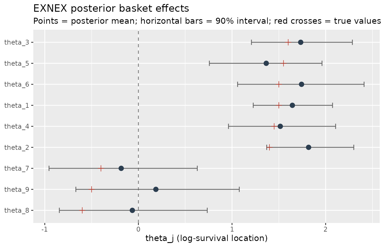
The responsive baskets (1–6) have tight intervals around their common value. The resistant baskets (7–9) are pulled partway toward the majority – their intervals lie between their true negative values and the positive exchangeable mean – illustrating that EXNEX reduces variance for discordant baskets but does not eliminate shrinkage.

Customizing the non-exchangeable prior per basket

Suppose the design protocol fixes baskets 7–9 as non-exchangeable a priori with a strong prior, so that they are not allowed to borrow. We can express this with basket-specific vectors for p_mix and v_nex:

fit_nex <- exnex_surv(
  Surv(time, event) ~ group + X1 + X2,
  data = d,
  priors = list(
    p_mix = c(rep(0.9, 6), rep(1e-6, 3)),   # baskets 7-9 almost surely non-exchangeable
    v_nex = c(rep(1e4, 6), rep(1e-4, 3))    # and tightly prior-ed around m_nex = 0
  ),
  iter = 1000, warmup = 500, chains = 1, seed = 7
)
fit_nex$resolved_priors$p_mix
#> [1] 9e-01 9e-01 9e-01 9e-01 9e-01 9e-01 1e-06 1e-06 1e-06

The resolved_priors report confirms the per-basket values were applied. With v_nex tiny, baskets 7–9 are pulled hard toward $m_{0j}=0$ regardless of the data, which is a strong (and here deliberately misspecified) assumption. This example is meant to illustrate the mechanics of basket-specific priors, not to recommend a particular prior.

Comparing EXNEX, EX, and No pooling

As a final illustration, compare the three model variants described above by overlaying their posterior basket-effect means:

fit_ex <- exnex_surv(
  Surv(time, event) ~ group + X1 + X2, data = d,
  priors = list(p_mix = 0.9999999),       # EX: full borrowing
  iter = 1000, warmup = 500, chains = 1, seed = 11
)
fit_np <- exnex_surv(
  Surv(time, event) ~ group + X1 + X2, data = d,
  priors = list(p_mix = 1e-6, v_nex = 1e4),  # No pooling
  iter = 1000, warmup = 500, chains = 1, seed = 13
)

means_of <- function(f) {
  s <- summary(f)
  setNames(s$mean, s$parameter)
}
compare <- data.frame(
  theta = theta_true,
  truth = theta_true,
  exnex = means_of(fit)[grepl("^theta_", names(means_of(fit)))],
  ex    = means_of(fit_ex)[grepl("^theta_", names(means_of(fit_ex)))],
  npool = means_of(fit_np)[grepl("^theta_", names(means_of(fit_np)))]
)
compare
#>         theta truth      exnex          ex      npool
#> theta_1  1.50  1.50  1.6446482  1.65289347  1.6689805
#> theta_2  1.40  1.40  1.8179920  1.84371052  1.8706961
#> theta_3  1.60  1.60  1.7337071  1.72777603  1.8047064
#> theta_4  1.45  1.45  1.5157022  1.50005465  1.5775365
#> theta_5  1.55  1.55  1.3655601  1.38489342  1.4235149
#> theta_6  1.50  1.50  1.7425843  1.73508263  1.8945620
#> theta_7 -0.40 -0.40 -0.1835898 -0.17724959 -0.5071769
#> theta_8 -0.60 -0.60 -0.0645867 -0.02207626 -0.3644995
#> theta_9 -0.50 -0.50  0.1867690  0.23799078 -0.1381373

exnex recovers the responsive baskets well and only partially shrinks the resistant ones; ex pulls every basket (including the outliers) strongly toward the common mean; and npool keeps each basket at its own noisy estimate. These three posterior summaries encode exactly the three borrowing strategies that EXNEX is designed to interpolate between.

Performance and validation

In the companion paper the data-augmented Gibbs sampler is compared with a marginalized Stan NUTS implementation of the same EXNEX model on 12,000 simulated trials (plus 1,000 TCGA-calibrated). On the four primary scenarios the two implementations produced essentially identical posterior summaries, but Gibbs averaged roughly 0.70–0.74 seconds per trial versus 16.96–17.53 seconds for Stan (a median runtime ratio of about 25 $\times$ ), and it delivered roughly ten times more bulk effective samples per second (3,854–4,032 versus 338–391). Operating characteristics (bias, RMSE, interval coverage) for EXNEX were close to nominal across scenarios and, under Mixed efficacy, EXNEX clearly outperformed both Complete pooling (which failed on the resistant baskets) and No pooling (which was inefficient on the responsive baskets). These figures are hardware- and implementation-dependent; they are quoted here to convey the order of magnitude of the speedup that data augmentation makes possible.

References

Neuenschwander, B., Wandel, S., Roychoudhury, S., & Bailey, S. (2016). Robust exchangeability designs for early phase clinical trials with multiple strata. Pharmaceutical Statistics, 15(2), 123–134.
Tanner, M. A., & Wong, W. H. (1987). The calculation of posterior distributions by data augmentation. Journal of the American Statistical Association, 82(398), 528–540.
Albert, J. H., & Chib, S. (1993). Bayesian analysis of binary and polychotomous response data. Journal of the American Statistical Association, 88(422), 669–679.
Eddelbuettel, D., & François, R. (2011). Rcpp: Seamless R and C++ integration. Journal of Statistical Software, 40(8), 1–18.
Sanderson, C., & Curtin, R. (2016). Armadillo: A template-based C++ library for linear algebra. Journal of Open Source Software, 1(2), 26.
Vehtari, A., Gelman, A., Simpson, D., Carpenter, B., & Bürkner, P.-C. (2021). Rank-normalization, folding, and localization: An improved $\widehat R$ for assessing convergence of MCMC. Bayesian Analysis, 16(2), 667–718.
Ney, V. (2026). Bayesian EXNEX survival models with data augmentation for basket trials. Manuscript.